Training algorithms are the core methods used to optimize neural network models. Each algorithm has unique characteristics and performance, making it essential to understand their strengths and weaknesses when choosing the right one for a specific task.

To simplify the learning process, we often abstract it into minimizing a loss function. This function typically includes an error term that measures how well the model fits the data, and a regularization term that controls model complexity to avoid overfitting.
The loss function's value depends on the model’s parameters—weights and biases. These can be combined into an n-dimensional vector, denoted as w. The figure below illustrates the loss function f(w).
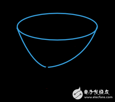
The minimum of the loss function, denoted as w*, represents the optimal set of parameters. By selecting any point in the parameter space, we can compute the first-order (gradient) and second-order (Hessian) derivatives of the loss function.
The gradient is a vector representing the direction of maximum increase: ∇f(w) = [df/dwâ‚, df/dwâ‚‚, ..., df/dwn]. The Hessian matrix contains the second partial derivatives: H_{i,j}f(w) = d²f/dw_i dw_j.
While many optimization techniques exist, they are often adapted for neural networks. One common approach is one-dimensional optimization, which helps determine the best step size along a given direction during training.
In practice, the training process involves iteratively updating the model parameters to minimize the loss. A key step is finding the optimal learning rate, which determines how much the parameters change at each iteration.
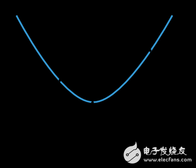
One-dimensional optimization methods like the golden section or Brent method are widely used to find the best step size η* within a range [ηâ‚, η₂], reducing the interval until it meets a predefined threshold.
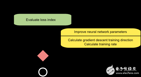
Multidimensional optimization methods, such as gradient descent, aim to find the global minimum of the loss function by adjusting the parameter vector w. At each step, the model updates its weights based on the gradient information.
The process begins with random initialization of parameters. Then, through repeated iterations, the loss decreases until a stopping condition is met, such as reaching a certain number of epochs or achieving a target loss value.
Now let's explore some of the most important training algorithms used in neural networks.

1. Gradient Descent
Gradient descent is one of the simplest and most commonly used training algorithms. It relies only on the gradient vector, making it a first-order method.
Let f(w_i) = f_i and ∇f(w_i) = g_i. Starting from an initial weight vector w₀, the algorithm moves in the direction of -g_i at each step, using a learning rate η_i to control the update:
w_{i+1} = w_i - η_i * g_i
The learning rate η can be fixed or adjusted dynamically during training. While many modern tools use fixed rates, adaptive strategies are becoming more popular due to their efficiency.
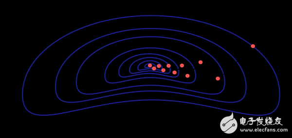
However, gradient descent has limitations. If the loss function has a narrow valley structure, the algorithm may take many iterations to converge. Additionally, while the gradient direction indicates the steepest descent, it may not always lead to the fastest convergence.
Despite these challenges, gradient descent remains a popular choice, especially for large-scale models with thousands of parameters. It requires minimal memory since it only stores the gradient vector, not the full Hessian matrix.
Automotive Connector Housing.
Automobile connector is a kind of component that electronic engineers often contact. Its function is very simple: in the circuit is blocked or isolated between the circuit, set up a bridge of communication, so that the current flow, so that the circuit to achieve the intended function. The form and structure of automobile connector are ever-changing. It is mainly composed of four basic structural components: contact parts, shell (depending on the type), insulator and accessories
Automotive Connector Housing
ShenZhen Antenk Electronics Co,Ltd , https://www.antenk.com